
Y. Liu1, C. Baldner1, R. Bogart1, R. Bush1, T. Duvall2, J. T. Hoeksema1, A. Norton1, P. Scherrer1, J. Schou2
1 Hansen Experimental Physics Laboratory, Stanford University, Stanford, CA 94305
2 Max-Planck-Institut für Sonnensystemforschung Justus-von-Liebig-Weg 3 37077 Göttingen
(Note: Table 2 is corrected on Feb 10, 2017)
HMI/SDO changed the scheme for collecting vector magnetic field measurements on 13 April 2016. Because we are now confident that data from the two HMI cameras can be successfully combined, the noise in the vector observations can be reduced by using all of the filtergrams from both HMI cameras.
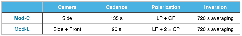
The new scheme, called Mod-L, changes the sequence of filtergram observations. The previous method, Mod-C, used the HMI front camera to collect filtergrams in circular polarization (CP, I ± V) at 6 wavelengths every 45 seconds, from which the Doppler velocity and other line-of-sight quantities were computed. In parallel, every 135 seconds Mod-C used the HMI side camera to obtain not only CP, but linearly polarized filtergrams (LP, I ± Q and I ± U) as well. Only side-camera filtergrams were used to compute the Stokes [I, Q, U, V] in Mod-C. In Mod-L the sequence for the front camera remains the same, while the side camera now collects only the linear polarizations.
Mod-L provides all of the filtergrams necessary to compute the Stokes parameters [I, Q, U, V] in 90 seconds, instead of the 135 seconds required for Mod-C. Thus Mod-L increases the maximum temporal resolution for measuring full Stokes parameters. At the same time, it decreases the noise because twice as many filtergrams are available. The 45s data products from the front camera are also improved; since there is no longer a 135s period in the instrument configuration, the corresponding peak in the Doppler power spectrum is now gone. The new 90s period is at the Nyquist frequency of the 45s-cadence Doppler data. The Stokes measurement is normally averaged over time (nominally 720 seconds) to derive [I, Q, U, V], and we now combine three times as many CP and 1.5 times as many LP measurements. Table 1 compares the Mod-C and Mod-L observations.
Table 1 | Measuring Stokes Parameters [I, Q, U, V]: Mod-C versus Mod-L.
Until recently, the HMI team was not confident that filtergrams from the two cameras could be calibrated with sufficient accuracy. Even after precise spatial alignment, combining filtergrams from two cameras to produce [I, Q, U, V] requires careful evaluation of differences in intensity, polarization, and wavelength to ensure that no systematic bias is introduced.
First, each filtergram needs to be scaled to normalize the average intensity for that cameras. It is done by calculating the ratio of the total intensities of two camera and applying this pixel-dependent ratio for rescaling. The intensity ratio between two cameras is about 1.05.
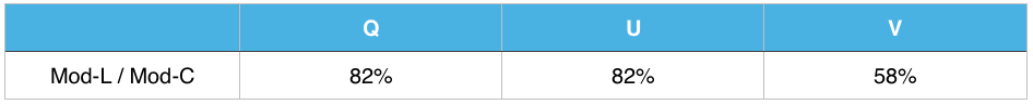
Second, we perform a preliminary evaluation of the polarization calibration by comparing the noise levels. The original polarization calibration model1 was determined using measurements from one camera only. We apply that polarization calibration model to derive Stokes [I, Q, U, V]. As expected just from photon statistics, the Mod-L noise level decreases by about 14% compared with Mod-C for the 720-sec averaged [I, Q, U, V] (see Table 2).
Table 2 | Noise in Stokes [Q, U, V]: Mod-C versus Mod-L.
This decrease of the noise in [I, Q, U, V] also reduces the noise in the inverted vector magnetic field data. Figure 1 shows mean values of the vector magnetic field components as a function of time from January 1 to May 15, 2016. Because the mean of the field magnitude (blue curve) is computed from all the pixels on the Sun’s disk and most pixels are in noise-dominated quiet Sun regions, this mean-field value is a fairly good proxy for the noise. The noise is reduced by ~8% from Mod-C to Mod-L.
Figure 1 | Temporal profiles of data mean of vector magnetic field (Yellow: inclination, Green: azimuth, Blue: field strength) from 1 Jan to 15 May, 2016. The orange curve indicates the camera, where camera = 1 represents the side camera (Mod-C), and camera = 3 means combining two cameras (Mod-L). While inclination and azimuth show no significant change between two observation modes, the mean of field strength decreases significantly. The field-strength mean is dominated by weak-field noise.
The polarization calibration model is also tested using the method described in ref. 2. The residuals of Stokes [Q, U, V] are very small, about 10-4, as shown in Figure 2. This confirms that the original calibration model works well with Mod-L data.
Figure 2 | The average Stokes [I, Q, U, V] quantities are computed for a 25-hour observation. The data are (1) rebinned to 256×256; (2) [Q, U, V] are divided by the corresponding Stokes [I]; (3) we average the near-continuum wavelengths 0 and 5; and (4) for each pixel, we take the median of the 25-hour data. The residuals of [Q, U, V] are very small, indicating current polarization calibration model works well with Mod-L data.
Finally, we need to determine if the two cameras require different wavelength-correcting phase maps. We perform this test using the Mod-C data that was collected with just one camera. We calculate the magnetic field in two ways, once using the phase map from the usual side camera and a second time with the front-camera phase map. The difference between the two vector field determinations is negligible: the difference between histograms of field strength is 0.1 G, the inclination difference is 0.1 degree, and the azimuth difference is 0.0 degree. There are no large-scale patterns visible in the difference images. Thus we conclude that it is acceptable for Mod-L to use the same phase map to correct filtergrams from both cameras.
Another end-to-end test is to compare the usual Mod-C vector field with the results of a pseudo-Mod-L sequence. To mimic the Mod-L sequence, we combine Mod-C filtergrams taken with the two cameras, i.e., we take two sets of CP from the front camera, and one set of LP from side camera to produce the Stokes [I, Q, U, V]. This is just like Mod-L, but we get one complete set every 135 seconds instead of every 90 seconds. Pseudo Mod-L data can be constructed from any existing Mod-C data and the results directly compared with the corresponding Mod-C data taken at the same time. Comparison shows that the resulting Stokes [I, Q, U, V] and the inverted magnetic field data from Pseudo Mod-L and Mod-C do not have any systematic bias.
Based on our analysis, we conclude that:
(1) The Mod-L observing sequence leads to lower noise in the Stokes [I, Q, U, V] and in the inverted 720-sec vector magnetic field data;
(2) Mod-L does not introduce any appreciable systematic bias;
(3) The current polarization calibration model works with Mod-L observation very well; and
(4) Using phase maps from front or side camera does not significantly impact the inverted magnetic field data.
Further tests may be required to adjust certain parameters in the HMI vector field analysis pipeline. In particular, with a lower noise level the threshold for selecting different methods of disambiguation in weak-field regions may need to be adjusted.
For additional details, see the SPD poster by Y. Liu et al.3
References
[1] Schou, J., Borrero, J. M., Norton, A. A., Tomczyk, S., Elmore, D., Card, G. L., 2012, SoPh, 275, 327
[2] Couvidat, S., Schou, J., Hoeksema, J. T., Bogart, R. S., Bush, R. I., Duvall, T. L., Liu, Y., Norton, A. A., Scherrer, P. H., 2016, SoPh, in press (http://arxiv.org/abs/1606.02368)
[3] http://sun.stanford.edu/~yliu/hmi/modL_Summary/YLiu_poster2016.pdf