
A.A. Norton1, E.H. Jones2, M.G. Linton3, J.E. Leake4
1 HEPL, Stanford University, Stanford, CA, 94305-4085, USA
2 The University of Southern Queensland, Toowoomba, QLD, 4350 Australia
3 US Naval Research Laboratory, 4555 Overlook Ave., SW Washington, DC, 20375, USA
4 NASA Goddard Space Flight Center, 8800 Greenbelt Rd., Greenbelt, MD, 20771, USA
Magnetic flux emergence into the solar atmosphere triggers transient events such as flares, coronal mass ejections and jets, as well as transports helicity via eruptions. Comparing the observed flux emergence process to numerical studies allows us to determine if the physics included in the simulations are realistic.
Some questions remain unanswered about flux emergence. For example, as the magnetic flux rises and expands greatly nearing the top of convection zone, does it simply slow its rise speed in the last few Mm or halt its rise altogether, thus needing an additional instability prior to emerging? Or, what percentage of flux remains trapped, just below the photosphere, unable to emerge into the atmosphere? While we don’t answer these ‘big picture’ questions in this paper, we quantify the emergence and decay rates of ten bipolar active regions using vector magnetic field data from HMI in order to better constrain the simulation conditions and understand the subsurface emergence process that we cannot observe directly.
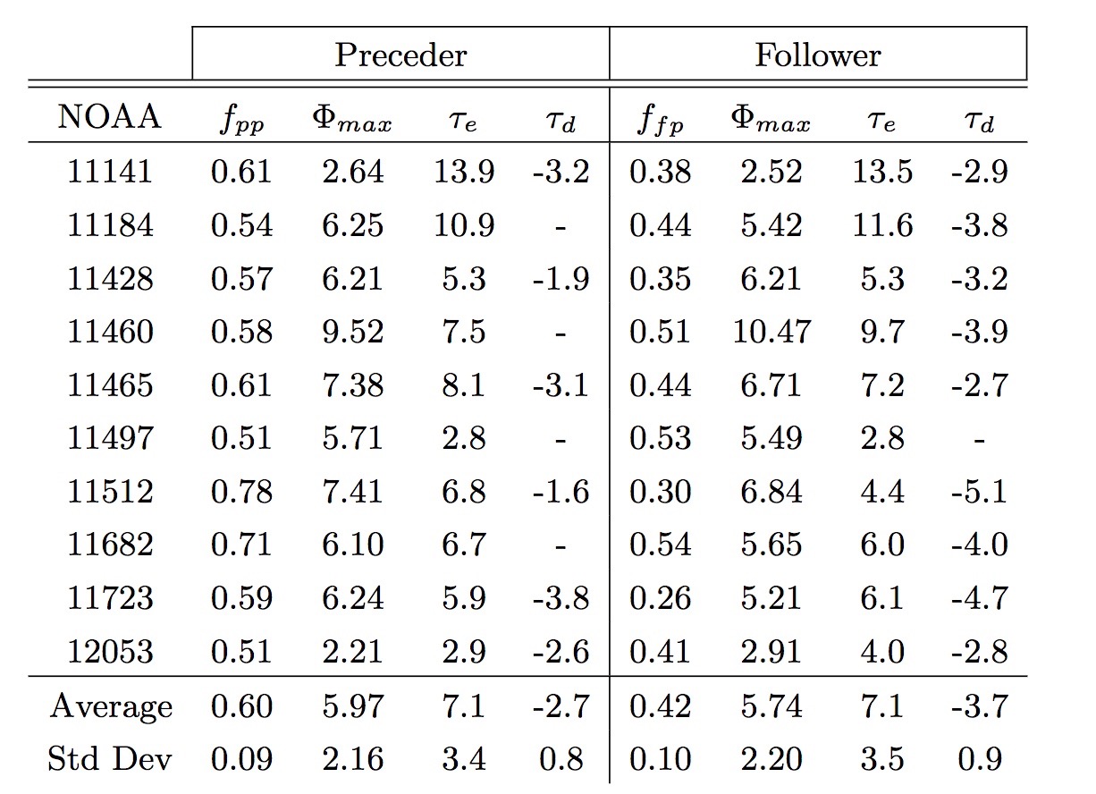
The bipolar regions examined in this paper contain an average signed flux of 5.9 × 10²¹ Mx emerging at 7.1 × 10¹⁹ Mx h-1 while decaying at half of that rate1, see Table 1. We define the beginning of active region emergence by the initial appearance of pores in continuum intensity. We require that the group emerge and begin to decay on the visible, Earth-facing side of the Sun. This criteria selects small- to mid-sized active regions. We apply a six-hour smoothing function. The flux emergence time is considered the period between when the flux reaches ten and ninety percent of the peak value. The emergence rate is simply the amount of flux emerged divided by the time. The decay period was defined as when the flux declined to ninety percent of the peak flux until it either reached ten percent or the slope was positive for two consecutive points in time. The ten regions show considerable scatter in emergence rates with a standard deviation of 3.5 × 10¹⁹ Mx h-1, half of the average rate. The observed decay rate is in reasonable agreement with the rate at which moving magnetic features are expected to carry away magnetic flux4.
Table 1|Results for preceder (p) and follower (f) flux within the SHARP patch regions by NOAA number. fpp is the ratio of flux within the preceder sunspots to the total preceder flux within the SHARP patch. ffp is the ratio of flux within the follower sunspots to the total follower flux within the SHARP patch. Φmax is the peak flux within the patch in 1021 Mx. τe (τd) is the flux emergence (decay) rate in 1019 Mx h-1. ‘-‘ indicates that the decay was not observed long enough to quantify the rate. The values in this table are calculated using a threshold of 575 Mx cm-2 in that magnetic flux values below this are not included in the analysis.
Our work is similar to several other observational studies2,3. However, our study is distinctive since [2] utilizes HMI line-of-sight data and reports maximum rates and [3] analyzes Hinode-SOT line-of-sight magnetic field for events observed for ~hours whereas we report average emergence rates determined from vector magnetic data after following the regions for approximately a week.
The observed rates of active region flux emergence are shown in context with a synthesis of other values in the literature, including ephemeral region emergence and simulation emergence rates, see Fig 1. Regions containing less flux exhibit slower emergence rates.
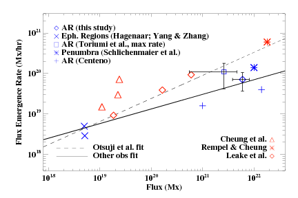
Figure 1| Signed flux emergence rates (Mx hr-1) as a function of peak magnetic flux (Mx) at the photosphere. The average emergence rate found in this study (◊) is compared with modeling results (Δ, *, ◊) and observations of ephemeral region (×), active region (+, []) and penumbral (*) emergence rates reported in the literature. The precise values plotted here as well as the reference papers in which they were published are summarized in Table 4 in [1]. We find that the emergence rate scales as a power law dependent on peak, radial flux values with an exponent of 0.36 (i.e., dΦ/dt ∝ Φmax0.36) (solid line)1. However, [3] report a flux emergence rate with a power law dependent on peak flux whose exponent is 0.57 (dashed line).
The difference in power law exponents reported herein and by [3] is likely due to the fitting of a composite set of values taken by multiple instruments over longer durations (days)1 compared to a single instrument observing regions for a shorter duration (hours)3.
Numerical modelling results (red symbols, Fig 1) clearly show that higher flux regions emerge faster. However, the observed values of dΦ/dt are smaller than those reported in simulation results by [5] and others. This may indicate a slower rise of the magnetic flux in the solar interior than what is captured or assigned in the simulations.
References
[1] Norton, A.A., Jones, E.H., Linton, M.G., & Leake, M.G., 2017, ApJ, in press (http://arxiv.org/abs/1705.02053)
[2] Toriumi, S., Hayashi, K., & Yokoyama, T., 2014, ApJ, 794, 19
[3] Otsuji, K., Kitai, R., Ichimoto, K., & Shibata, K., 2011, PASJ, 63, 1047
[4] Hagenaar, H.J., & Shine, R.A., 2005, ApJ, 635, 659
[5] Rempel, M., & Cheung, M.C., 2014, ApJ, 785, 1