
Xudong Sun1,2 (for the HMI Team)
1. Institute for Astronomy, University of Hawaiʻi at Mānoa, Pukalani, HI 98768
2. W. W. Hansen Experimental Physics Laboratory, Stanford University, Stanford, CA 94305
New HMI 96-minute vector magnetograms are now available. Deep averaging reduces noise and enhances long-lived magnetic structures.
HMI has been observing the Sun for over 10 years. The routine, 12-minute-cadence vector magnetograms[1] are widely used by the solar community. The data series temporally averages several sets of Stokes parameters to enhance the signal-to-noise ratio (SNR). At HMI’s 720 km resolution, the 12-minute cadence is generally sufficient for resolving most photospheric dynamics. In 2017, the HMI team released the high-cadence (90 or 135 s) vector magnetograms[2]. At the expense of SNR, the new data series is designed for studying more rapid evolution such as during major eruptions.
We have created a new, deep-averaged vector magnetogram data series for HMI. It is suitable for studying the weaker but more stable magnetic fields, such as those in the polar region. This 96-minute cadence series (hmi.B_5760s) has the same format as the routine 12-minute series, and are processed with nearly identical pipeline options[3]. The corresponding Stokes profile data series is also available (hmi.S_5760s). The temporal averaging is performed over a tapered window of about 2.4 hours. The nominal times (center of averaging window) of the 15 frames each day are fixed at 00:00, 01:36, 03:12, etc. The data series provides a nice continuation from the 96-minute SoHO/MDI line-of-sight magnetograms. It will be processed upon request.
Figure 1|Comparison of Stokes Q maps. Top: Averaged Stokes Q from the 96-minute data, normalized by (inferred) local continuum, for the south polar region at 2015.03.04_12:48:00_TAI. Bottom: Stokes Q for 12-minute data.
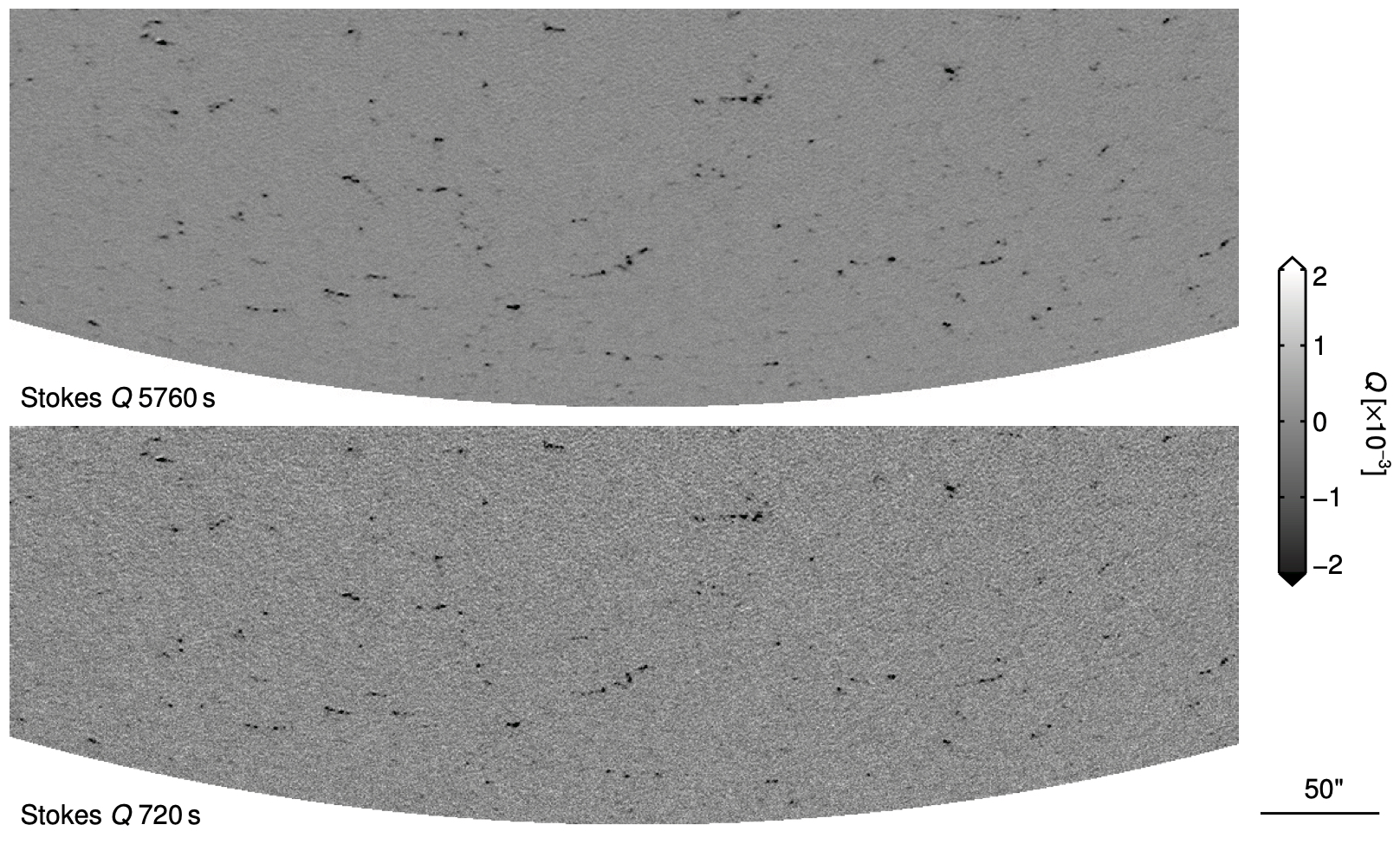
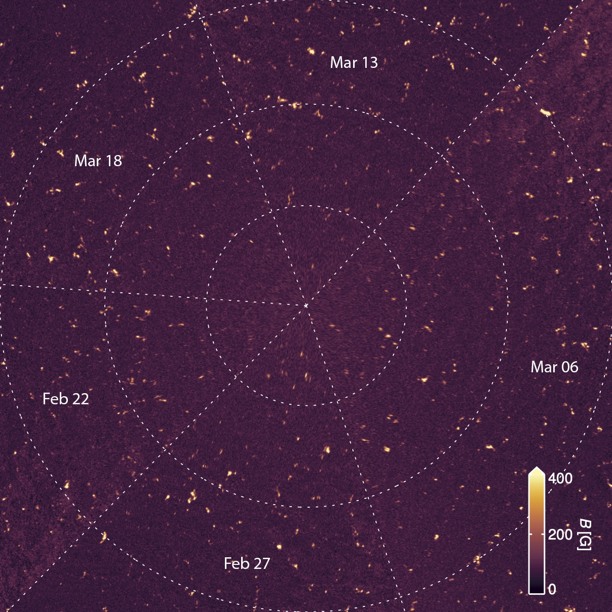
As illustrated by Fig. 1, the deep averaging significantly increases the SNR of the Stokes: strong field patches really stand out from the background. We note that evolution can also cause differences between these two versions: shorter-lived or fast-evolving features may be absent from, or appear smeared in the 96-minute data. Fig. 2 showcases the inferred magnetic field strength B over the entire southern polar region based on the 96-minute data. This stereographic map is constructed from 5 single magnetograms taken several days apart during February and March 2015. Strong field patches of several hundred G are clearly visible all the way to the pole.
Figure 2| The HMI polar magnetic landscape. The map shows the inferred magnetic field strength of the southern polar region in a stereographic projection. The circles indicated latitudes at -80, -70, and -60 degree. The map is constructed from five 96-minute vector magnetograms taken at 12:48_TAI on 2015-02-22, 02-27, 03-06, 03-13, and 03-18.
We have performed preliminary analysis of the southern polar field. We estimated the photon noise of the Stokes parameters (Q, U, V) and include only pixels whose maximum absolute Q, U, or V are greater than 5 times their respective photon noise. As shown in Fig. 3, the total number of pixels satisfying the selection criteria significantly increases in the 96-minute data. Most additions correspond to a weaker field strength at about 100 G, which is below the noise
Figure 3| Histogram of magnetic field in the polar strong-field patches. We study a single magnetogram at 2015-03-04_12:48_TAI. We include only pixels between -60 and -85 degree latitude, and between -85 and +85 degree longitude. See main text for the SNR selection criteria.
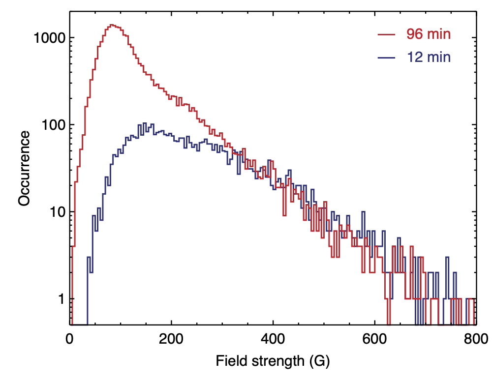
floor in the 12-minute data. We do not find any kilo-Gauss field identified in the Hinode/SP observation[4]. This is not surprising, because (1) HMI assumes a unity filling factor for the Stokes inversion[1] so the returned value is effectively the mean flux density, and (2) the lower spatial/spectral resolution of HMI is known to cause differences in inversion results[5]. We caution that these averaged Stokes signals need to be interpreted with care.
References
[1] Hoeksema, J. T., Liu, Y., Hayashi, K., et al. 2014, SoPh, 289, 3483
[2] Sun, X., Hoeksema, J. T., Liu, Y., et al. 2017, ApJ, 839, 67
[3] “HMI 96-Minute Vector Magnetograms” (http://jsoc.stanford.edu/data/hmi/b96m/)
[4] Tsuneta, S., Ichimoto, K., Katsukawa, Y., et al. 2008, ApJ, 688, 1374
[5] Leka, K. D. & Barnes, G. 2012, SoPh, 277, 89