
Luca Bertello, Alexei A. Pevtsov, Gordon J.D. Petrie
National Solar Observatory, 950 Cherry Ave., Tucson, AZ
Synoptic maps are routinely used to display the distribution of various physical quantities over the entire solar surface. Such maps are indispensable, for example, in representing global/large scale properties of solar magnetic fields in the photosphere and corona including location of active regions and complexes of activity (active longitudes or activity nests), coronal holes, chromospheric filaments, and the heliospheric neutral sheet. Synoptic maps of the photospheric magnetic field are currently used as the primary drivers for all coronal and solar wind models. These maps are created by merging together a series of magnetic observations spanning at least a full solar rotation (about 27 days)1. As for any other measurements, the full disk magnetic observations that form the basis for the synoptic maps are subject to noise in the measured parameters. The noise could depend on the instrument characteristics (e.g., type of detector, telescope aperture, pixel size), observing conditions (e.g., atmospheric seeing for ground-based instruments or disturbances in orbital parameters for space‐borne platforms) and other similar factors. Moreover, since the synoptic charts are constructed by averaging a contribution of individual images with smaller pixels into maps with larger pixels, there are additional statistical uncertainties. Until now, however, magnetic synoptic maps were produced without corresponding uncertainties and were essentially treated by modelers as noise-free input.
In a recent paper2, Bertello and collaborators at NSO have made a first attempt to estimate some of these uncertainties and evaluated their impact on coronal and heliospheric models. They found that accounting for the statistical uncertainties arising from the distribution of image pixels contributing to each bin in the synoptic map may produce a noticeable change in the results obtained from these models. This will enable forecasters to put uncertainties into their space weather forecast.
Figure 1:Photospheric magnetic flux density distribution (top) and corresponding uncertainty map (bottom) for Carrington rotation 2137. Both charts were computed using Fe I 630.15 nm SOLIS/VSM full disk magnetic observations. The top image has been scaled between +/- 30 Gauss to better show the distribution of the weak magnetic flux density field across the map. The actual flux density distribution, however, covers a much larger range of field values – up to several hundred Gauss.
Figure 1 illustrated an example of a photospheric magnetic flux density synoptic chart, and the corresponding uncertainty map. The charts were computed using Fe I 630.15 nm SOLIS/VSM full disk longitudinal magnetic observations covering Carrington rotation 2137 (May – June 2013). The figure shows that uncertainties are larger in areas associated with strong magnetic fields of active regions. To test how the uncertainties in a synoptic magnetic flux map may affect the calculation of the global magnetic field of the solar corona, we computed a Potential-Field-Source-Surface (PFSS) model of the coronal field for a Monte Carlo simulation of 100 Carrington synoptic magnetic flux maps generated from the uncertainty map.
Figure 2: Top, the PFSS neutral line (thin black lines) and positive/negative open field footpoints (red/blue pixels) are shown for CR 2137. The open field footpoints correspond to coronal holes and the neutral line represents the heliospheric current sheet. Bottom, the 100 model neutral lines for a Monte Carlo simulation of Carrington synoptic magnetic flux maps generated from the uncertainty map are over-plotted. Solid red/blue indicates pixels where 100% of the models have positive/negative open field, white represents footpoints where all models have closed field, and stronger/fainter coloring indicates where a larger/smaller fraction of the models have open field.
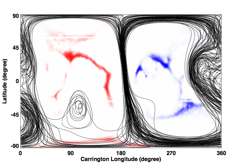
Figures 2 illustrates the result of this experiment. The CR 2137 global coronal field, shown in Figure 2 (top), is typical of coronal structure around solar maximum: the global dipole is tilted at an angle close to 90 degrees with respect to the rotation axis. The positive/negative coronal holes are confined to the eastern/western hemisphere and the neutral line encircles the Sun passing close to both poles. In the original CR 2137 model the neutral line is mostly confined to the western hemisphere, whereas in a significant number of the models in the Monte Carlo simulation the neutral lines are shifted into the eastern hemisphere. In a subset of the simulations a secondary compact, closed neutral line appears near 90 degrees longitude, -45 degrees latitude. The coronal hole distributions of the Monte Carlo simulations closely resemble the distributions in the original models in general. However, the faint coloring of some of the coronal hole structures in the bottom panel indicates that some large coronal hole structures, e.g., the most northerly and southerly red patches in the eastern hemisphere, are absent from a significant proportion of the models.
Spatial variance maps will likely improve the diagnostic value of existing coronal and heliospheric models by providing quantitative estimates of observational uncertainties. Thus they will open opportunities to refine modelers’ scientific conclusions and space-weather forecasts.
References
[1] Harvey, J. and Worden, J., 1998, in Balasubramaniam, K.S., Harvey, J.D, Rabin (eds.) Synoptic Solar Physics, ASP Conf. Ser., 140, 155.
[2] Bertello, L., Pevtsov, A.A., Petrie, G.J.D., Keys, D., 2014, Solar Physics, 289, 2419.