A. Sainz Dalda^1,2
1. Stanford-Lockheed Institute for Space Research, Palo Alto, CA 94304,USA.
2. High Altitude Observatory, Boulder, CO 80301, USA.

We have compared the vector magnetic fields derived from observations with the HMI instrument onboard SDO, with those observed by the SP instrument onboard Hinode. We have obtained relationship between the components of magnetic vectors in the umbra, penumbra, and plages observed in 14 maps of NOAA AR 11084. Similarly, we have also investigated the relationship between apparent longitudinal magnetic flux, B_app, total magnetic flux, Φ, and total unsigned magnetic flux, Φ̂, obtained by both instruments^[1].

To obtain a better understanding of the role played by different actors in the inversion of the Stokes parameters, we have transformed SP data into observables comparable to those of HMI (S2H data). Thus, we compare HMI vs SP, HMI vs S2H, and S2H vs SP data to quantify statistically the effect of the inversion code, filling factor(FF), spatial and angular resolutions, disambiguation of the azimuth, and spectral lines used by both instruments. Table 1 shows the combination of the data and actors used in our investigation.

Table 1| Cross-inversion setups. See Ref [1] for details.

Table 2 shows the relationship between the Cartesian coordinates of B^HMI and B^SP in the umbra, penumbra, and the strong and weak plages. In the umbra and penumbra, these coordinates are strongly related following a linear relation. In the strong and weak plages, the linear relationship is moderate and weak, respectively.

Table 2| Comparison between the Cartesian components of the vector magnetic field observed by HMI and SP.

Figure 1 shows a visual comparison between the spherical components of the magnetic field recovered from the inversions on HMI, SP and S2H data treated with different FF (either variable or equal to 1), different spectral sampling, and different disambiguation codes (AZAM^[2] and DIS^[3]). The actor playing the most important effect in the comparison between the magnetic field recovered by HMI and SP is the FF. The second important actor is the spectral sampling, and finally, the spatial sampling. The disambiguation method used to obtain the azimuth has an important influence in the plages. We suggest studying the possibility to use a similar disambiguation code on both data.

Figure 1| Components of the vector magnetic field in spherical coordinates observed by the HMI, SP , SP with FF=1, S2H , S2H with FF=1, and HMI in the sunspot. The disambiguated azimuth is shown in the 4th row. See Ref [1] for more details.

Figure 2| Same as Figure 1, but for the plages.

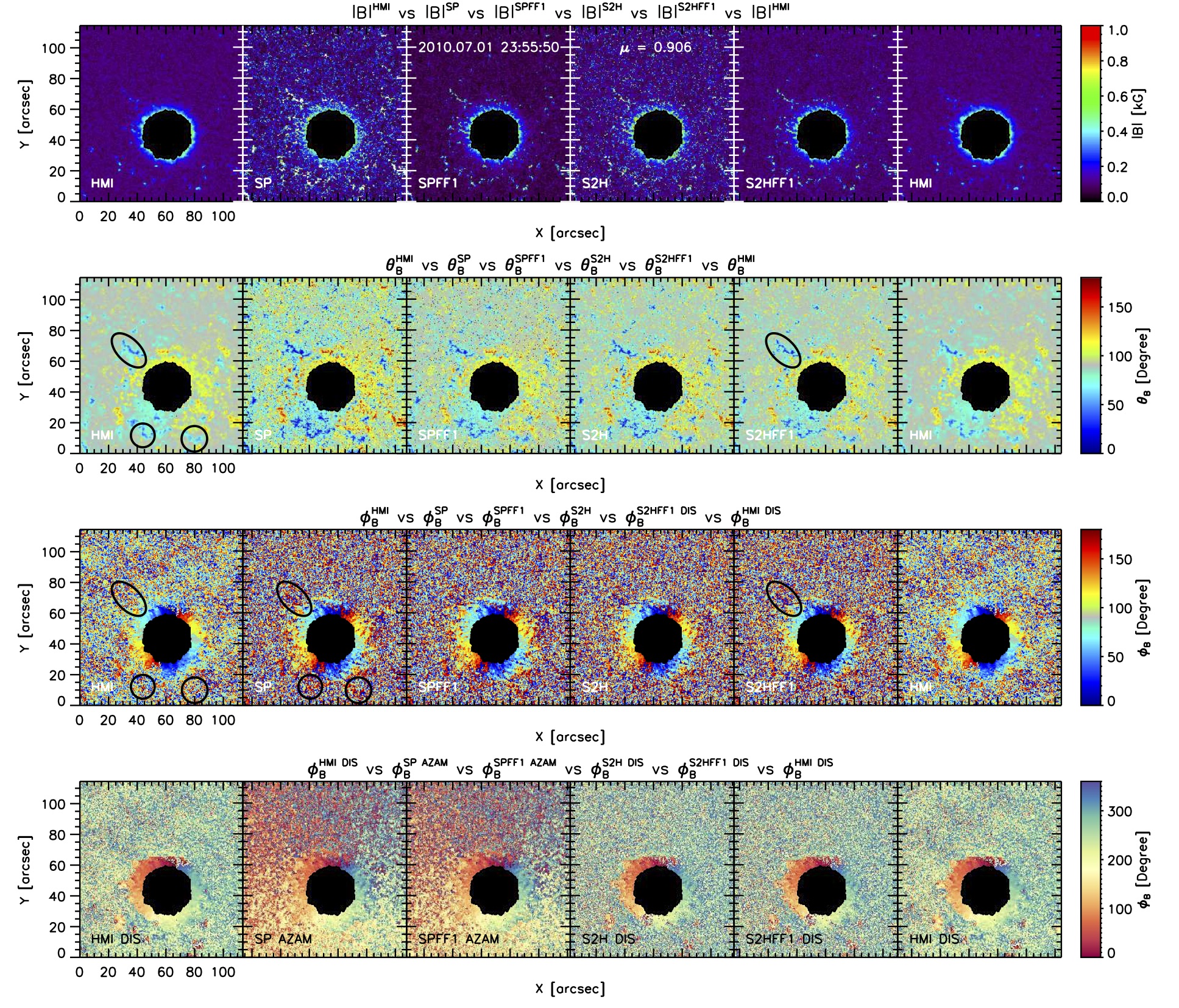
Table 3 shows the relationship between the B_app, Φ, and Φ̂ calculated from the HMI and SP data. In the umbra, HMI “sees” slightly lower values than the ones seen by SP. In the penumbra, B_app “observed” by HMI is slightly lower than the one observed by SP. However, HMI sees in the penumbra a Φ and Φ̂ with higher values (~15%) than the ones seen by SP. In the plages, HMI sees ~ 30% of B_app and Φ, and ~ 10% of Φ̂ seen by SP. If we average the values of Φ̂ in the field of view, i.e. without paying attention to the solar feature, the averaged value of Φ̂ (57%) agrees with the one reported by Thalmann et al.^[4] (54%). Nevertheless, our averaged horizontal component of B is ~60%, while their value is 81%. This difference may be due either to the selection method of the pixels considered in the comparison or the number of maps studied in each investigation (1 map in Ref [4] versus 14 in our study) and their location in the solar disk.

Table 3| Comparison between B_app, Φ, and Φ̂ for the HMI and SP.

To understand the impact of the FF in the values recovered from the inversions on the same data, we have inverted the SP data using the same inversion code with exactly the same actors except the FF (see Table 4). In the umbra, the recovered values are roughly the same, i.e. the FF variable is ‘fixed’ to 1 by the code in the umbra. In the penumbra, there is an overestimation of ~ 5% in the values obtained considering FF = 1 (as SPFF1 and HMI do) with respect when the FF is a variable (as SP does). In the strong plage, an inversion considering an FF fixed to 1 yields an 80% of the B_app, and ~ 60% of Φ and Φ̂ of these values produced by an inversion considering an FF variable. In the weak plage, these percentages are 74 % of B_app, 60 % of Φ, and 44% of Φ̂.

Table 4| Similar to Table 3, but between SP and SP with FF =1.

References

[1] Sainz Dalda, A., 2017, ApJ, 851, 111S
[2] https://www2.hao.ucar.edu/csac/csac-magnetic-field-disambiguation
[3] Hoeksema, J. T., Liu, Y., Hayashi, K., et al. 2014, Sol. Phys., 289, 3483
[4] Thalmann, J. K.; Tiwari, S. K.; Wiegelmann, T., 2013, ApJ , 769, 59